Home + About me + E-mail me + My slide rules
No more than thirty years ago [the late 1960s], slide rules were everywhere. Unlike many instruments, instead of being steadily improved by the new electronic technology, they were completely wiped out; sharing the fate of mechanical cash registers and clockwork watches. It seems that few people today know how to use a slide rule; most of my contemporaries who learned at school have forgotten.
I had my first rule when I was about eleven, bought for me by my father to stop me fiddling with his, and had several while at school and university. Like everyone else, I bought an electronic calculator when they became affordable around the early 1970s, and used it and its many successors for real work, but I still retain my fascination for the simple old method, and I still carry a slide rule and use it occasionally.
Put a slide rule on the table next to a modern scientific calculator. One of them consists of half-a-dozen or so pieces of plastic with marks on, the other contains the equivalent of millions of transistors, a few score of electrical switches, a chemical power source, a display screen, and probably at least as many pieces of plastic with marks on as the other. Yet the calculator is faster, more accurate, easier to use and cheaper. Amazing what technology can do, but also slide rules were always far more expensive than they ought to have been. Though, of course, you can make yourself a slide rule in a few minutes (see here); try that with a calculator!
When slide rules were a reasonable means of performing calculations quickly and cheaply, most science students were taught to use one at school. Mostly, though, students seem to have been taught just the basic methods for using the slide rule, and not the more efficient advanced methods, nor much about how it all works, and therefore how to develop technique. In this note I intend to set down what I've learned about it, before I forget it too!
A slide rule is a simple mechanical device to perform multiplication and division.
The slide rule's operation is based on the mathematical property of logarithms, that:
log(a) + log(b) = log(a*b)
or in words that finding the product of two numbers is the same as finding the number whose logarithm is the sum of the logarithms of the two numbers.
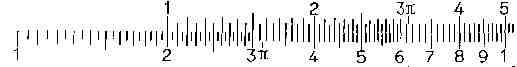
Here is a diagram of a basic slide rule, set up for multiplication by 2:
In the lower half of the picture is a scale running from "1" through "2" and "9" back to "1" again. Consider the interval between the two "1" marks as a unit interval; within this interval each number is plotted at a position proportional to its logarithm. For example, "1", whose logarithm is 0, is plotted right at the start of the interval; "2" (log 2 = 0.3) is plotted just under a third of the way along; "3" (log 3 = 0.48) is near the middle, and "10", whose log is 1, is at the end of the interval. ("10" is written as "1" for reasons which might become clear later.)
The upper scale is an identical scale, but shifted to the right by 0.3 (log 2). With these two scales positioned like this, it is possible to see how simple multiplication works. Note that the "1" on the upper scale is aligned with "2" on the lower scale, and also that "2" on the upper scale is aligned with "4" on the lower scale, this is showing that 2 times 2 gives 4. From the definitions of the scales, the distance from the left-hand "1" mark to the "2" mark on both scales is log 2 = 0.3, and it can be seen that the distances on the two scales add together to make 0.6, at which point on the lower scale we find the number whose logarithm is 0.6, that is 4.
With the scales at the same position, any other number may be multiplied by two, simply by finding the required number on the upper scale, and reading down to the lower scale. For example 2*3=6 or 2*4.5=9.
This is a photo of a typical slide rule:
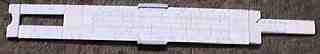
It consists of three parts, the stock, the slide and the cursor.
The stock is normally made either as two separate strips joined at the ends by bridge pieces (as shown), or as a single piece with a recess cut out for the slide to run in. In either case, the slide slides within the stock; tongues on the slide engage with grooves in the stock to keep it in line. The cursor slides along the stock, and has a clear window with a fine line marked perpendicular to the slide motion. It is used to record positions representing intermediate results, or to project from one scale to another where they are not adjacent. The rule shown above is double-sided, with a wrap-around cursor, but many are single-sided.
The material is commonly high-quality plastic, but older rules tend to be wooden, and expensive ones are often metal. Wooden ones are faced with a thin layer of plastic to take the scale. Plastic scales are engraved and filled with ink; metal rules may have a white background and scale marks printed or silk screened on.
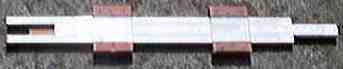
This is an old wooden Faber single-sided rule, fitted with two cursors:
It is conventional to put the scales that we have already seen, with one unit interval for the whole length of the rule, at the lower sliding edge on the front of the rule, that is the sliding scale is on the bottom edge of the slide, and the fixed scale on the upper edge of the lower part of the stock. These scales are conventionally known as "C" and "D" respectively. Their position is shown on this image of the left-hand end of the rule:
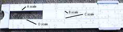
The diagram also shows two more scales, "A" and "B", at the upper slide edge. These scales are plotted with a half-size unit interval, so each scale runs from 1 to 100 in the same length that C and D run from 1 to 10. We'll come onto them, along with the dozens of other possible scales, later.
Slide rules come in various sizes, and the size refers to the length of the unit interval on the C and D scales. This length is typically 125mm for pocket rules, 250mm for most rules or, rarely, 500mm. The two common sizes are usually called 12-centimetre (or five-inch) and 25-centimetre (or ten-inch) rules. Some rules, not necessarily American made, have the unit length exact in old-fashioned units, for example 254mm for a "ten-inch" rule. As we shall see later, the length of the rule is important as it controls the maximum accuracy that can be achieved. The most accurate slide rules abandon the linear slide and use helices to achieve scale lengths of several metres.
We've already seen an example of multiplication above, but before going on let's introduce some conventions to describe in words how to set the rule. The form C:4 will be used to mean the position 4 on scale C. C:I will mean the index of the C scale, which might be the 1 or the 10 mark. In these terms, the process of multiplying 2 by 2 as shown above would be written as: bring C:I over D:2; answer found on D opposite C:2.
We've seen how to multiply 2 by 2, but how about 20 by 200? The answer is that it is done the exact same way. Except in certain special cases, slide rule calculations are done ignoring powers of ten. Of course, the correct power of ten is required in the answer, and usually this is supplied either by knowing the approximate answer, or by working out the answer very roughly on paper and using the slide rule just to supply more accuracy. So, to multiply 20 by 200, we work out:
20 * 200 =
(2.0 * 10) * (2.0 * 10²) =
(2.0 * 2.0) * (10¹ * 10²) =
4.0 * 10³ = 4000
using the slide rule for the significant figures and mental arithmetic for the powers of ten.
How do we multiply 3 by 5? Try the same procedure as before, and put C:1 over D:3. This puts C:5, where we look for the answer, off the end of the D scale. In this case, we make use of the fact that we do not care what power of ten we include in the answer. There's nothing under C:5, but if we look exactly one unit length to the left of C:5, we'll find the result for 5 * 3 / 10, because subtracting one unit length is equivalent to dividing by 10. This process is done in practice by using C:10 instead of C:1, which moves the slide one unit to the left (let's call this "reversing the slide"). Bring C:10 over D:3, then read the answer, 1.5, under D:5.
There are rules which can be used to work out the power of ten for the answer given the powers of the multiplicands and the exact way the slide is moved, but in my opinion they are not much help except in simple cases. For example, let's take 25 * 600. First reduce the arguments to the range 1..10 by extracting powers of ten, so:
25 * 600 =
2.5 * 6.0 * 10¹ * 10² =
2.5 * 6.0 * 10³
Then work out the figures on the slide rule. The power of ten for the answer is the sum of the powers of the arguments, plus one for every time we use the C:10 mark to start a multiplication. Here we have to use the C:10 mark over D:2.5, to find 1.5 on D as the answer under C:6. So the power of ten of the answer is 4, and the full result is 1.5 * 104 = 15000. There is a corrresponding rule for division (see below) where the power of ten of the answer is decreased by one every time the result is found under C:10 instead of C:1. As I say, I think it's easier to approximate the result overall than to keep track of the number of slide reversals.
Because the scales are logarithmic, the size of the divisions changes as you go along the scale. Typically, a 25cm rule might have divisions every 0.01 from 1 to 2, every 0.02 from 2 to 4, then 0.05 from 4 to 10. This takes a little practice to read quickly. Also, to add to the confusion, the labelling is often abbreviated. For example, the subdivisions between 1 and 2 are often labelled just 1 to 9, which really means 1.1 to 1.9. In all cases, you are expected to estimate by eye down to about one-fifth of a division. Almost all scales have a special mark for pi, and often other constants as well.
Want to try some examples? How about 1.91 * 2.42 (=4.62); 5.13 * pi (=16.12); 1.01 * 1.01 (=1.02).
Division is based on the formula:
log(a) - log(b) = log(a/b)
so uses subtraction of distances rather the adding we used for multiplication. We can see this with the same setting of the rule as we used for multiplication by 2, which also shows the position for, say, 6 divided by 3 gives 2. You can see how the distance 1..3 on C, which is log 3 = 0.48, is subtracted from the distance 1..6 on D, which is log 6 = 0.78, to leave the distance 1..2 on D, which is 0.3 = log 2
The basic rule is: align the divisor (number to be divided by) on C with the dividend (number to be divided) on D, and read the answer under the index of C. For example, slide C:3 over D:6 and read the answer, 2, under C:1.
As with multiplication, for some pairs of numbers, C:1 will be off the end of the D scale; then the answer will appear under C:10. This will actually be ten times the answer, as we're reading one unit interval to the right, but as usual we are not concerned with powers of ten.
Another example: 365/12. Set C:1.2 over D:3.65 and read the answer 30.4 under C:1. In this case, as we're working out the average number of days in a month, we can guess the powers of ten!
Other examples: 1.6 / 3.5 (=0.457); 150000000 / 1.61 (=93200000); 64 / 5 (=12.8).
When aligning two numbers, neither of which are on an exact division, it may be helpful to place the cursor on the dividend on D, then bring the divisor on C under the cursor line. Where one or more of the arguments are on exact divisions it may be more accurate not to use the cursor, but even then it can be helpful to put it nearby to keep the eye focused on the right part of the scale.
By a chained calculation, I mean something like a*b*c, or a*b/c.
When there are repeated multiplications, the cursor is used to hold the result of one calculation on D, while the index on C is brought up for the next. For example, let's do 2*3*4*5. Place C:1 over D:2, then bring the cursor up to C:3, thus marking the first intermediate result (2*3=6). Then bring C:10 under the cursor line and move the cursor to C:4, marking the second intermediate (2*3*4=24). Then bring C:10 again under the cursor line, and read the final result under C:5 (2*3*4*5=120). (The powers of ten rule would say two reversals of the slide, so add two powers, so result = 1.2*10² = 120.) Note that each multiplication involves one slide movement and one cursor movement.
Repeated divisions work much the same way. Let's try 1/(2*3*4). First align D:1 with C:2, then place the cursor at C:10, marking first intermediate (1/2 = 0.5) on D. Then bring C:3 under the cursor and move the cursor to C:1, which is the second intermediate (1/6 = 0.167). Finally bring C:4 under the cursor and read the result 0.0417 under C:10. (The rule would say C:10 used for result twice, so deduct two powers, so result = 4.17*10-2 = 0.0417.) Note again that each step requires a slide and a cursor movement.
Alternating multiplication and division is the most efficient sequence when only C and D scales are available. To see this, let's try (4*5)/(8*0.125). Calculated in the order in which it is written, it would go: C:10 over D:4, cursor to C:5, C:8 under cursor, cursor to C:10; C:1.25 under cursor, result D:2 under C:1. That's 6 movements, including reading the result. Alternating it would go: C:8 over D:4, cursor to C:5, C:1.25 under cursor, result under C:1 = D:2. That's four movements, including reading the result.
Working this through, you can see why it's more efficient to alternate, as division leaves the intermediate result under C:I, which is where it is needed for multiplication, so there's no need to mark it with the cursor. Similarly, multiplication leaves the result marked with the cursor on D, which is where it is needed for the next division. Of course, it might work out that a division leaves the slide set so that the next multiplier on C is off the end of the D scale, in which case the cursor has to be moved and the slide reversed, reducing the saving. Other scales, such as CF and DF help to reduce this. Also, other techniques using reciprocal scales can make repeated multiplication or division as efficient as alternating.
Some examples to try: (2.5 * 4.6 * 1.7) / (0.125 * 456 * pi) (=0.109); (2/3) * (11/13) (=0.564).
Before starting with more scales, a note about names. I haven't seen a rule yet that doesn't have C and D scales on the lower sliding edge on the front. All but one of mine has A and B scales at the upper sliding edge on the front. These scales are almost universally labelled by the letters A, B, C and D on the left-hand end of each scale. Beyond these, any combination of scales may be found, and most of the other scales have names which either denote their function, such as S for sine, or their relationship to C or D, such as CI for C inverse. These names for these scales also seem to be pretty universal. The old wooden rule in the picture above has only ABCD scales on the face, in the conventional place but unlabelled, though the S, T and L scales on the back of the slide are labelled.
In addition to the names on the left of each scale, most rules have the derivation of each scale, from the base CD scales, shown by a formula at the right-hand end. In these fomulae, the C and D scales are represented by x, so they both have x at their right-hand ends. Scales A and B, with half the unit interval, are both labelled x² (x-squared). To see why this is so, think about the mid-point of the A-scale, which represents 10. This point is vertically above the mid-point of the D-scale, say at some reading x. Now as this is the mid-point, log(x) = 0.5, or x=sqrt(10). Reading backwards, sqrt(10) on D reads onto A as 10. This is true for any position on D, so any number on D reads onto A as its square. Thinking about it another way, the factor of two scale change in linear distance terms between A and D represents a squaring by the equation:
log(a) * 2 = log(a²).
Apart from this use of calculating squares and square roots, the A and B scales can be used for multiplication and division in the same way as C and D, but of course with reduced accuracy, though this is compensated by the reduced need to reverse the slide. For example, to do our previous example of 2*3*4*5 on A and B scales we could do: B:1 over A:2; cursor to B:3; B:1 under cursor; cursor to B:4; B:100 under cursor; answer under B:5 = A:120.
In finding square roots by reading from A to D, it is important to think carefully about powers of 10, as a difference of one power on the A scale translates to sqrt(10) on D, which is not just a matter of adding a zero! The rule is to reduce the number to a value between 1..100 and an even power of ten, take the root and then put back half the power of ten. Some examples:
sqrt(16000) =
sqrt(1.6 * 10000) =
sqrt(1.6) * sqrt(10000) =
1.265 * 100 =
126.5
sqrt(160000) =
sqrt(16 * 10000) =
sqrt(16) * sqrt(10000) =
4 * 100 =
400
sqrt(0.00025) =
sqrt(2.5 * 10-4) =
sqrt(2.5) * sqrt(10-4) =
1.58 * 10-2 =
0.0158.
Reading from A to D is of course done with the cursor. In calculations that require a square or a square root, it is often possible to get clever and do part of the calculation on AB and part on CD, crossing when the second-power operation is called for. For example, to calculate 8 * (.2*16)² proceed thus: C:1 over D:2; cursor to C:1.6; B:1 under cursor, cursor to B:8 and read the result at A:82. Of course, great care is needed if a square root is to be taken, to ensure the required even power of ten exists.
There is usually only one K scale, on the stock, marked x³ (x-cubed), with three logarithmic cycles in the space of one on the C scale, running from 1 to 1000. Reading from D to K gives the cube, and from K to D the cube root. As with square roots, it is necessary to get the powers of ten under control. With cube roots, the number must be between 1..1000, and the power of ten a multiple of 3. An example:
cube-root(10-16) =
cube-root(100 * 10-18) =
cube-root(100) * cube-root(10-18) =
4.64 * 10-6 =
0.000 004 64.
I have one odd rule that has two K scales (K and K') at the upper sliding edge on the reverse, so that calculation can be carried on after cubing. Given the limited accuracy of these scales, I don't see why anyone would want to.
CI is very often present; DI is unusual. The scales are marked 10/x or sometimes 10:x at the right-hand end. They are plotted with the same unit interval as C, but the marks are plotted at 1-log(a) instead of at log(a) for C, so they look the same as C or D, but run backwards from 10 to 1. CI is on the slide, and DI is on the stock. Their formula is:
1-log(x) = log(10)-log(x) = log(10/x)
and reading from C to CI or from CI to C produces the reciprocal, ignoring powers of ten.
The main use of CI especially is not to find reciprocals per se, but for speeding up chained calculations. Remember that multiplication by x is equivalent to division by 1/x, and you can see that is it possible to turn a multiplication operation, where C:I is placed, into a division-like operation, where the operand is placed, if that is more convenient in a chain. Let's run that 2*3*4*5 again, using this technique: put the cursor on D:2; put CI:3 under the cursor; move cursor to C:4; put CI:5 under cursor; read result under C:1 (=120). This is only five movements, including reading the result, as opposed to six the other way, and there was no need to think about reversing the slide.
As you work through a calculation, at each stage you can make a tactical decision whether to proceed by the obvious multiplication or division, or whether to use the CI scale and the opposite operation, based on convenience, and positioning for the next operation.
I've seen no use for DI.
These scales are marked pi-x, and when present are often at the upper sliding edge on the reverse. They are normal unit-length scales, but shifted to the right by log(pi), so that crossing from say D to DF gives a multiplication by pi, and from DF to D gives a division by pi. This can be useful in itself, but the prime purpose of these scales is to facilitate chained calculations and tables. As pi is close to sqrt(10), these scales are shifted by about half a basic unit; this means that until the slide is more than half-way out, there is always at least one incidence of each value on C or CF that is aligned with D or DF, and by carrying on the calculation on the appropriate pair slide reversals can be eliminated.
This is particularly obvious when setting up a table. Say that we want to convert some prices from pounds to marks, with a conversion factor of *2.7. We set the rule so that C:1 is over D:2.7, then by moving the cursor along, any price in pounds on C can be converted to marks on D, so 3 pounds converts to 8.1 marks. However, pound amounts from about 3.8 to 10 on the C scale are off the end of the D scale, so normally we would have to keep reversing the slide, to put C:10 over D:2.7, depending on the amount to be converted. But, without moving the slide, we see that on CF amounts from about 3.2 to 11 pounds are over DF, so we can convert 7 pounds on CF to 18.9 marks on DF.
Or try (2/3) * (11/13) again, it's easier with CF and DF: C:3 over D:2; cursor to CF:1.1; CF:1.3 under cursor; answer opposite CF:1 (=0.564).
When working with CF and DF, it's important to keep in mind whether the cursor is set to a value on D or on DF. When you're looking for a value on C, you can just as well use CF, but once you've chosen which and placed the cursor, you must use the corresponding scale for the next operation. If you've read from CF to a value on DF, saving that DF value with the cursor, you must place the next division operator on CF under the cursor, not C, or if the next operation is a multiplication, you must use the CF scale's index. If this sounds complicated, it's probably because it is. Few people who don't use a slide rule all the time would bother with CF and DF except for tables.
The logarithm scale looks different from all other scales because it is a linear scale, like a ruler. It is labelled log x. It is usually marked 0.0 to 1.0 along the unit interval, so reading from C to L gives the fractional part of the logarithm, from the definition of the C scale. The integer part of the logarithm must be supplied, as the power of ten. For example, log 400: C:4 lies over L:0.602; 400 is 4 * 10²; so log 400 is 2.602. Similarly, reading the other way gives 10x, so for 102.3: 102.3 = 100 *100.3; L:0.3 corresponds to C:1.995; so 102.3 is 199.5.
If a rule had two L scales, one on the slide and one on the stock, it would be possible to do simple addition, but pretty pointless.
These scales are basically just look-up tables for common trigonometric functions. They are usually marked in degrees, or in some cases degrees and minutes. Their range is fairly restricted. These scales are the first that we have met that cannot do arithmetic on their own, they are just tables, and what's more they are not invariant under factors of ten. Each scale relates to just one value on the corresponding base scale, so to cover a wider range of angles, there have to be more of them.
The commonest set is probably ST, S and T, defined as arc(0.01x) (ST), arcsin(0.1x) (S) and arctan(0.1x) (T). These scales would usually be on the stock, and x in the formulae is the value of the D scale. Arc is used to stand for arcsine or arctangent when the angle is so small that they are indistinguishable at the resolution of a slide rule. The ST scale shows the angles whose sines are in the range 0.01 (opposite D:1) to 0.1 (opposite D:10), roughly 0.6 degrees to 6 degrees. The S scale covers 6 degrees to 90 degrees (sines in the range 0.1 to 1) and the T scales cover about 6 degrees to 45 degrees (tangents in the range 0.1 to 1). Sometimes T is called T1, and an extended tangent scale, T2, is supplied for angles from 45 to about 84 degrees; this has formula arctan(x). Often the scales are also marked with red numbers running the opposite way, to remind the user that cos(x) = sin(90-x) and cot(x) = tan(90-x).
The scales are mostly used for looking up trig functions, but they can also be incorporated into calculations; to work out 5*sin(25) put C:I above S:25 (using the cursor); read the result on D opposite C:5 (=2.115). The blooper to avoid is to try calculations using the angles: the trig scales are not themselves logarithmic, you cannot calculate 2*arcsin(.5) directly. You must first calculate arcsin(.5) by cursor to D:5, read S:30; manually transfer this to D:3 (for 30); then multiply by 2 in the usual way on C and D.
Another common pattern is to have just two trig scales, on the back of the slide (of a single-sided rule); they are brought into use by pulling the slide right out and flipping it over. In this case, the upper scale, usually S, is marked with reference to the B scale which it temporarily replaces, and the lower scale, T, is marked with reference to the C scale which it replaces. So the T scale is the same as before, but the S scale runs from 0.6 degrees to 90 degrees, with 6 degrees in the middle, and the left-hand half of it also acts as an ST scale for tangents of small angles. This arrangement is sometimes convenient for calculations, removing the need to carry across with the cursor, but loses accuracy on S and is generally only found on low-spec rules. These rules often have small windows on the back which allow sine and tangent look up to be done without flipping the slide over; you line up your angle on say the S scale with the mark in its window, then read the corresponding sine on the front under A:100.
For angles less than 0.6 degrees, the sine and tangent are so close to the angle in radians that conversion is done by multiplication by pi/180. There is often a mark at C:1.745 or its reciprocal C:5.73 to make this easier. Sometimes there are other marks for angles in minutes and seconds.
Another possibility is the P scale, for Pythagoras, which is scaled as sqrt(1-(0.1x)²). This can be used to convert the sine of an angle to its cosine without going through the angle (in the range 0.1 to 1 only), but I've never had cause to use it.
Some Thornton rules have idiosyncratic trig scales, which instead of directly looking up the trig functions of an angle instead look up the ratio between those functions and the angle itself. These scales are very short, which allows sine, tangent and both inverses to fit into the length of one conventional scale. Their formula is difficult to write in the conventional format where the scale value is given as a function of x, the other way round giving the value of x at which the angle T is plotted they are x = T/sinT for SD and x = T/tanT for TD. To find the sine of T: set T on SD over T on D and read result on D under C:I. The inverse trig scales read to CI scale so that a division operation actually performs a multiplication. To find the angle whose tangent is x: set x on D aligned with x on ITD and read the result on D under C:I. These scales give a better range of angles, effectively automatically using sin(x) ~= x for small angles, and are claimed to give better accuracy everywhere, but like most clever tricks few users will remember how to use them from one time to the next.
The log-log scales are another set that are not power-of-ten invariant, so again there is a whole family of them, the posher the rule, the more of them there are, though I've not seen more than eight on one rule. The basic formula of LL0 is e0.001x, of LL1 e0.01x, of LL2 e0.1x and of LL3 ex. The basic formula of LL00 is e-0.001x, of LL01 e-0.01x, of LL02 e-0.1x and of LL03 e-x. The commonest set is just LL2 and LL3, and in general the positive exponent ones are commoner than the negative.
The scales are used for taking powers and roots of numbers, and for taking logarithms to other bases. They have the disadvantage that, except for a limited range of numbers, they are horribly approximate, as the scales are very compressed for the larger values of x.
The LL scales can be used as straight look up tables, to find natural logarithms and powers of e. For example, to find ln(pi): use the cursor to project LL3:3.14 to D (=1.14).
Unlike the trig scales, it does make sense to do arithmetic with the values on the log-log scales. The numbers on the LL scales are plotted at their logarithmic position, onto a logarithmic scale, so using the single-log C-scale alongside the double-log LL scales is equivalent to multiplying the logs of the numbers on the LL scales, which means exponentiation. The formula is:
log(ln(x)) + log(a) = log(a*ln(x)) = log(ln(xa))
(where 'x' is the reading on the LL scale and 'a' the reading on C) so to find 32.5: set C:1 over LL3:3 and read the result (=15.6) on LL3 opposite C:2.5. To find 29: set cursor on LL2:2; set C:10 under cursor; read result on LL3 under C:9 (=~500). Note how, because using C:10 instead of C:1 loses a power of ten, we had to read the result from the next higher log-log scale to get the power of ten back again.
Another calculation possible on the LL scales is to take log to any base. Remembering that, say log2(6) is the power that we have to raise 2 to to get 6, and that raising to a power is like multiplying the LL scale by the C scale, place C:10 over LL2:2, and then place the cursor over LL3:6; we find the required result on C at 2.58. Again we used C:10 rather than C:1, but compensated by reading from LL2 to LL3. Another example: log5(20) = 1.86 can be done using the values on C directly, and entirely on the LL3 scale, and another: log2(1.2) = 0.263 can be done entirely on LL2, but use of C:10 rather than C:1 makes the result one tenth of the C scale reading.
The LL0x series scales do the same thing, only for numbers less than one. If they're not there, you can often use the LLx scales instead, by taking the reciprocal of the numbers. So to find e-2 we can read from D:2 to LL03 to find 0.135, or read to LL3 at 7.4 and return the result 1/7.4 =0.135.
These are a feature of some Thornton slide rules, and effectively provide an LL1 scale with just a very short extra scale at the end of the rule, to the left of the A scale. The LL1 scale is very useful for interest rate calculations as it covers ratios from 1.01 to 1.11, or 1% to 11%. The markings of LL1 are quite close to D scale markings in that 1.01 is just left of D:1, 1.04 a little further left of D:4 and so on. The little differential scale just provides a convenient way of offsetting this small displacement. Setting the extra "Y" cursor against 4% on the differential scale and reading D against C:4 reads the equivalent result to setting the cursor to LL1:1.04 and projecting to D.
At the next level down, for the LL0 scale from 1.001 to 1.01, the marks are so close to the D scale that they can be used equivalently; some Faber rules use this to share the D scale with LL0.
These are pretty esoteric. Their function is to provide increased accuracy for multiplication and division, at the expense of considerable extra complexity. Typically, they occupy both sliding edges on one side, stretching a single 1..10 unit range into the total length of both. The lower scales are called W1 (where D would be) and W1' (instead of C); the upper set are W2 (instead of A) and W2' (instead of B). Their formulae are sqrt(x) for W1 and W1'; sqrt(10x) for W2 and W2'.
A diversion on the subject of accuracy. We have seen that logarithmic scales have the property that any given linear distance corresponds on the scale to a fixed multiplier, that's how multiplication works. So any error in reading, which is likely to be the same physical distance wherever we are on the scale, corresponds to a constant ratio error in the reading, and a constant percentage error. This means that the accuracy of a slide rule, depending as it does mainly on the human eye reading and estimating between engraved marks, is better the longer the unit cycle. Suppose we take the reading error to be 0.1mm, which would be pretty good, then on a 250mm rule this represents a ratio error of 100.1/250 = 1.00092 (you can do that calculation on a slide rule if you have LL3 and LL0 scales!) or about 0.1%. For a 125mm it's 0.2%, and for a 500mm it's 0.05%. This factor is applied for each slide or cursor operation, so for 6 operations expect no better than 0.6% on a 250mm. Greater accuracy can be got only by longer scales or finer divisions, and presumably a microscope to see them with.
So, a cheap way to double your accuracy is to double the scale length, but given the inconvenience of carrying or using the rule this cannot go very far. Hence the compromise of double-length folded scales.
W scales are not too bad if you keep your wits about you. The lower W1 scales start at 1 and stop at a red mark where 10 on D would have been, we'll call this W1:R. The upper W2 scales start at a red mark called W2:R and run up to 10. The red marks are important, as they get used in place of the normal scale indexes. Think of them as marking sqrt(10), so when they are used they inject spurious factors of sqrt(10). However, as the W2 scales are offset by sqrt(10) from W1 (they're offset one half of a unit length, remember), the spurious sqrt(10) factors can be taken out again by crossing the rule. So we get a basic principal: if your calculation used a normal index, read on the same side; if it used a red mark, cross the rule for the answer.
Let's try an example: 2*2. If you set W1':1 over W1:2, W1':2 is off the end. So, set W1':R over W1:2 instead, then move the cursor to W1':2. Now, because we used a red mark, don't read the result on W1, but cross the rule and read it on W2, to find the result 4. It works!
You don't have to use the red marks, you can use the proper index marks on the opposite side and line up using the cursor, then it's even more obvious that as you crossed over to set the index you should cross back to read the result. I think the red lines are easier.
Let's try a division, say 2/6. 2 is on W1 and 6 is on W2, so set the cursor to W1:2 and bring W2':6 under the line; read the result 0.333 on W2 opposite W2':R. We use the red mark as we crossed sides when we set up the division.
That's about it, as there are no short-cut facilities, no equivalent of CF and DF or CI; also no trig functions or other fancy scales based on the W scales. You can do basic multiplication and division more accurately, that's all.
I've only seen these on an American Pickett rule. They are effectively double and triple length scales, but on the stock only so they can't be used for high-accuracy multiplication and division. The do provide more accurate squaring, square rooting, cubing and cube rooting than a normal rule.
The only scales not yet mentioned that I have on any of my rules are dedicated electrical ones. These operate with special marks on the ABCD scales to calculate voltage drop in copper cables and the efficiency of an electric motor or generator. They are so specialised that without the instructions it's easier to do the calculations on the general scales, unless it's something you do every day.
Some makers of slide rules pack the cursor with extra lines. As the fixed spacing between two lines on the same scale corresponds to a multiplication factor, simple conversions can be arranged, provided the factor is close enough to one to fit onto the cursor. A common one is kilowatts to horsepower, at 735 watts or 746 watts depending on country of origin.
Another, almost universal, one is to read from 2 on D to pi on A; this one combines two factors and a squaring to calculate pi*(x/2)², or the area of a circle of diameter x.

Home + About me + E-mail me + My slide rules